Dimensionality reduction based on angular-based features

Here, we demonstrate the application of various dimensionality reduction methods to visualize angular features in a reduced-dimensional space. As an example, we will focus specifically on three selected PED ensembles for N-terminal SH3 domain of Drk protein.

PED00156: This ensemble consists of conformations generated randomly and optimized through an iterative process.
PED00157: This ensemble includes conformations generated using the ENSEMBLE method, which creates a variety of realistic conformations of an unfolded protein.
PED00158: This ensemble is a combination of conformations from the RANDOM and ENSEMBLE pools

1- The first step is to extract the specific feature we wish to analyze.

analysis.extract_features(featurization='phi_psi')

PARAMETERS:

The extract_features method of the analysis object is designed to extract specific features from the loaded ensembles.

The parameters we can set to extract different angular data are:

“featurization”: Choose between “phi_psi”, “a_angle”, “tr_omega”, and “tr_phi” for angular data.

“min_sep”: Minimum separation distance for “tr_omega”, and “tr_phi” methods. Default is 2.

“max_sep”: Maximum separation distance for “tr_omega”, and “tr_phi” methods. Default is None.

2- The second step is choosing dimensionality reduction method and hyperparameters.

After selecting the feature to extract, we can apply various dimensionality reduction methods using the reduce_features function. The parameters that can be set for this function are numerous and vary depending on the chosen reduction method.

analysis.reduce_features(method='umap', n_neighbors = [10, 50, 100, 150, 200, 250] ,circular=True, range_n_clusters=range(2,10,1));
# In this example we chose umap as the dimensionality reduction method and other hyperparameters with respect to that.

PARAMETERS:

“method”: Choose between “pca”, “tsne”, “kpca” and “umap”.

“fit_on”: If method is “pca” or “kpca”, specifies on which ensembles the models should be fit. The model will then be used to transform all ensembles. The default is None

ADDITIONAL PARAMETERS (Based on the chosen method):

PCA:

“num_dim”:Number of components to keep. Default is 10.

For more information, visit the scikit-learn documentation.

t-SNE:

“perplexity_vals”: A list of perplexity values. The default is [30]. This list can contain multiple values, but each value must be less than the total number of conformations. If a list of values is provided, the package will determine the optimal perplexity by evaluating all combinations of cluster numbers and perplexity values, selecting the one that achieves the best clustering based on the Silhouette score.
“metric”: Metric to use. Default is “euclidean”.
“circular”: Indicates whether to use circular metrics. This should be set to True when analyzing angular data. The default value is False.
“n_components”: Number of dimensions of the embedded space. Default is 2.
“learning_rate”: Learning rate. Default is ‘auto’.
“range_n_clusters”: Range of cluster values. Default is range(2, 10, 1).

For more information, visit the scikit-learn documentation.

KernelPCA:

“circular”: Indicates whether to use circular metrics. This should be set to True when analyzing angular data. The default value is False.
“num_dim”: Number of components to keep. Default is 10.
“gamma”: Kernel coefficient. Default is None. If gamma is None, then it is set to 1/n_features

For more information, visit the scikit-learn documentation.

UMAP:

num_dim: Number of dimensions for the reduced space. Default is 2.
n_neighbors: Number of neighbors to consider for each point in the input data. This can be a list of numbers. Default is [15]
circular: Indicates whether to use circular metrics. This should be set to True when analyzing angular data. The default value is False.
min_dist: The minimum distance between embedded points. Default is 0.1.
metric: The metric to use for distance calculation. Default is ‘euclidean’
range_n_clusters: Range of cluster values to consider for silhouette scoring. Default is range(2, 10, 1).

For more information, visit the UMAP documentation.

3- The third step is the visualization of the results.

After performing dimensionality reduction on your data, you can visualize the results using various methods from the visualization module. The primary function for representing the output of t-SNE and UMAP is the dimensionality_reduction_scatter, which creates a scatter plot of the reduced data in 2D or 3D space, effectively showcasing cluster separation and relationships.

For PCA and KernelPCA outputs, additional specialized visualization methods are available to provide deeper insights:

pca_2d_landscapes: Generates a 2D landscape plot of the principal components, helping to identify clusters and patterns in the reduced space.
pca_cumulative_explained_variance: Displays the cumulative explained variance by the principal components, which helps assess how much variance is captured by the chosen number of components.
pca_1d_histograms: Produces 1D histograms for individual principal components, offering insights into the distribution of the data along each component.
pca_rg_correlation: Plots the correlation between the principal components and the radius of gyration (Rg), which can help reveal structural properties.
pca_residue_correlation: Visualizes the correlation between individual residues and the principal components, providing a more detailed understanding of how specific regions contribute to the overall structural variability.

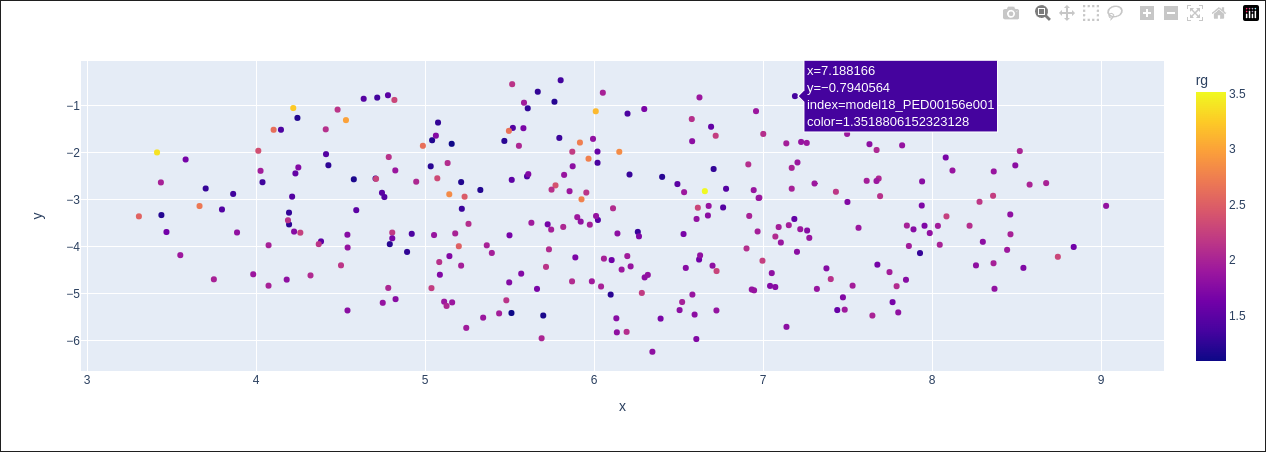
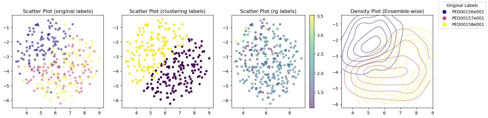
In the first example you can see the results of UMAP on the phi and psi angles as features

vis.dimensionality_reduction_scatter(color_by='rg', kde_by_ensemble=True, size=20, n_comp=2, plotly=True);

PARAMETERS:

color_by: Specifies the feature used to color points in the scatter plot. Options include: “rg” (radius of gyration), “prolateness”, “asphericity”, “sasa” (solvent accessible surface area), and “end_to_end”. Default is “rg”.
save: If True, the plot will be saved to the data directory. Default is False.
ax: A list of Axes objects to plot on. If None, new axes are created. Default is None.
kde_by_ensemble: If True, a separate KDE (Kernel Density Estimate) plot will be generated for each ensemble. If False, a single KDE plot for all concatenated ensembles will be produced. Default is False.
size: Specifies the marker size for scatter plot points. Default is 10.
plotly: If True, an interactive Plotly scatter plot is generated. Hovering over points reveals model numbers in the ensemble, 2D embeddings, and the selected ensemble property based on the color_by value. Default is False.
n_comp: If the dimensionality reduction method yields 3 components, a 3D plot will be visualized; otherwise, a 2D plot is generated.

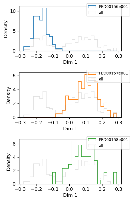
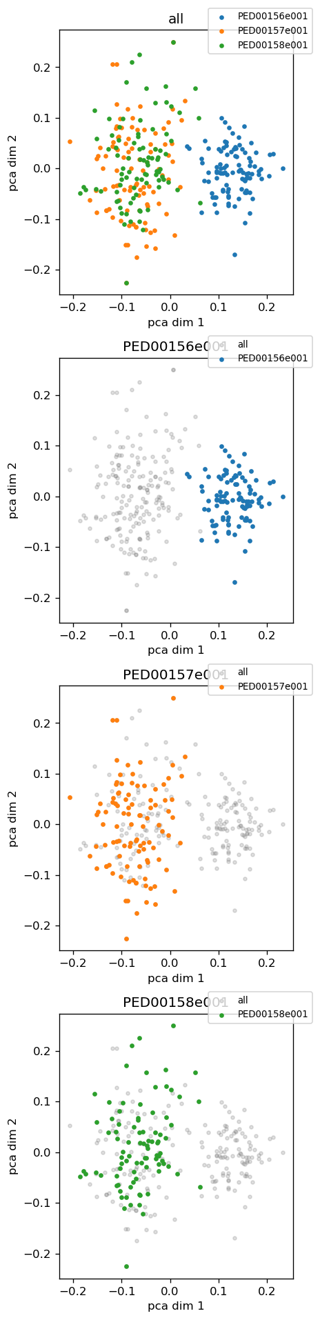
In the second example we are using KernelPCA as the dimensionality reduction method to show phi and psi features. Then using pca_2d_landscapes method we can plot the result.

analysis.reduce_features(method="kpca", circular=True);
vis.pca_2d_landscapes(save=False)

You can also generate a 1D histogram to visualize the distribution of the data across different dimensions or components. This provides an overview of how the data is distributed along specific axes, helping to identify patterns or trends in the dataset.

vis.pca_1d_histograms(sel_dim=1)