Global analysis
In this demo we show how we can extract and visualize the global properties from conformational ensembles using IDPET.
The global properties that studied here are : Radius of Gyration, Asphericity, Prolateness, End-to-End distance, Flory scaling exponent and Global SASA.
To illustrate the output of our functions, we have chosen the analysis of the SH3 protein as an example. The graphs we present are related to the analysis of this protein, comparing three distinct ensembles downloaded directly from the Protein Ensemble Database (PED): PED00156, PED00157, and PED00158. These ensembles represent structural states of the N-terminal SH3 domain of the Drk protein (residues 1-59) in its unfolded form, generated with different approaches to initialize pools of random conformations.
PED00156: This ensemble consists of conformations generated randomly and optimized through an iterative process.
PED00157: This ensemble includes conformations generated using the ENSEMBLE method, which creates a variety of realistic conformations of an unfolded protein.
PED00158: This ensemble is a combination of conformations from the RANDOM and ENSEMBLE pools, offering greater conformational diversity.
Initialize the analysis
from dpet.ensemble import Ensemble
from dpet.ensemble_analysis import EnsembleAnalysis
from dpet.visualization import Visualization

ensembles = [
 Ensemble('PED00156e001', database='ped'), #The ensemble derived from Random pool
 Ensemble('PED00157e001', database='ped'), #The ensemble derived from Experimental pool
 Ensemble('PED00158e001', database='ped')]

data_dir = '/path/to/directory/save_results' # Add the path to a directory you wish in order to save the analysis

analysis = EnsembleAnalysis(ensembles, data_dir)
analysis.load_trajectories() # load the trajectories which already downloaded from PED for upcoming analysis

vis = Visualization(analysis=analysis) # make the visualization object for visualizing ensemble features
Radius of gyration
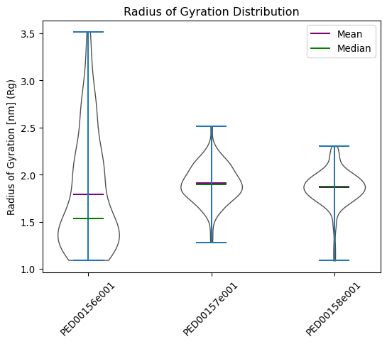
The radius of gyration of a protein is the square root of the mean square distances of the protein residues from the protein’s center of mass. It is therefore a measure of the compactness of its three-dimensional structure.
“bins”: Number of bins for the histogram; default is 50.
“hist_range”: A tuple defining the min and max values for the histogram; if None, uses the data range.
“multiple_hist_ax”: If True, plots each histogram on a separate axis.
“violin_plot”: If True, displays a violin plot; default is False.
“location”: It allows you to specify whether to calculate and use the mean (‘mean’) or the median (‘median’) or (‘both’) as the reference value.
“dpi”: The DPI (dots per inch) of the output figure; default is 96.
“save”: If True, saves the plot as an image file; default is False.
“ax”: The matplotlib Axes object(s) on which to plot; if None, new Axes object(s) will be created.
vis.radius_of_gyration(violin_plot=True, color='white', location='both')
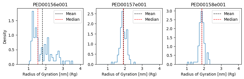
vis.radius_of_gyration(multiple_hist_ax=True ,hist_range=(0.5,4) ,location='both', bins=40)
End to end distance
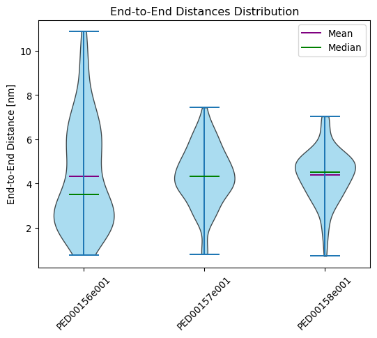
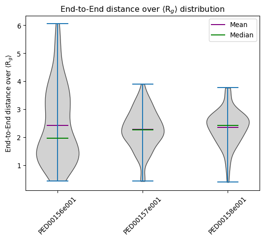
The end_to_end_distances function is designed to visualize the distributions of end-to-end distances in molecular structure trajectories. The end-to-end distance refers to the distance between the first and last atom in a molecular chain, a parameter often used to understand the overall size of conformations of a molecule.
“rg_norm”(bool,optional):If set to True, normalizes the end-to-end distances based on the average radius of gyration.[The default value is False]
“bins”(int,optional): Defines the number of bins for the histogram of distances. More bins provide a more detailed distribution, but it may be noisier.[The default value is 50]
“hist_range”(tuple, optional):A tuple specifying the minimum and maximum values for the histogram. If not specified (None), it uses the minimum and maximum values present in the data.
“multiple_hist_ax”: If True, plots each histogram on a separate axis.
“violin_plot”(bool,optional):If set to True, the function will generate a violin plot of the distances. [The default value is True]
“location”: It allows you to specify whether to calculate and use the mean (‘mean’) the median (‘median’) or (‘both’) as the reference values.
“save” (bool, optional):If set to True, the generated plot will be saved as an image file. [The default value is False]
“ax” (plt.Axes, optional):The axes on which to plot. [The default value is None]
The end-to-end distances are computed by selecting the Cα atoms from each ensemble’s trajectory and calculating the distance between the first and last Cα atoms in each frame:
Where:
\(\mathbf{r}_{\text{start}}\) is the position of the first Cα atom.
\(\mathbf{r}_{\text{end}}\) is the position of the last Cα atom.
This example generates a violin plot of the end-to-end distances and both showing means and medians.
vis.end_to_end_distances(violin_plot=True, color='skyblue', location='both')
It is also possible normaize the end-to-end distances based on the average radius of gyration, generating violin plots that include the means.
Where RG is the mean Radius of Gyration of the trajectory.
vis.end_to_end_distances(violin_plot=True, color='silver', location='both', rg_norm=True)
Asphericity distribution
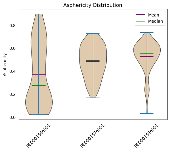
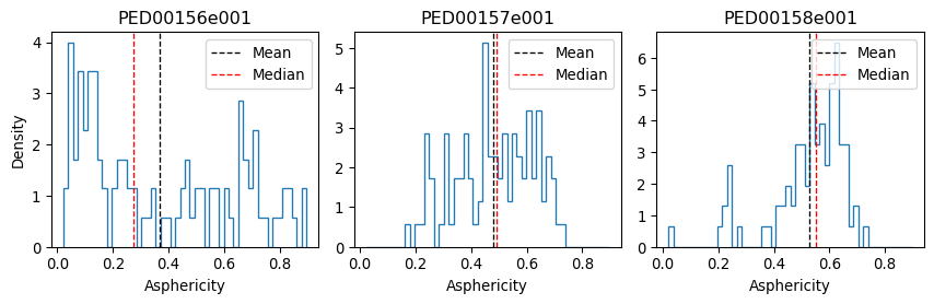
Asphericity is a measure of how much a molecule deviates from a perfect spherical shape. It indicates the extent to which a molecule is elongated or flattened compared to an ideal sphere. A protein with an asphericity value greater than zero is generally more elongated or less symmetric than a sphere.
To calculate asphericity, the gyration tensor is first computed for each frame of the trajectory. The eigenvalues of this tensor, which represent the principal moments of inertia and provide insights into the molecule’s shape and symmetry, are then sorted in ascending order.
Finally, asphericity is calculated using the following formula:
where \(\lambda_{1},\lambda_{2},\lambda_{3}\) are the sorted eigenvalues of the gyration tensor.
“bins”: Number of bins for the histogram; default is 50.
“hist_range”: A tuple defining the min and max values for the histogram; if None, uses the data range.
“violin_plot”: If True, displays a violin plot; default is True.
“location”: It allows you to specify whether to calculate and use the mean (‘mean’) or the median (‘median’) as the reference value.
“save”: If True, saves the plot as an image file; default is False.
“multiple_hist_ax”: If True, plots each histogram on a separate axis.
“ax”: The matplotlib Axes object on which to plot; if None, creates a new figure and axes.
vis.asphericity(violin_plot=True, location='both', color='tan')
vis.asphericity(violin_plot=False, location='both', multiple_hist_ax=True)
Prolatness distribution
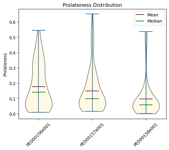
Prolateness is a measure of a molecule’s shape, indicating how elongated it is relative to its transverse dimensions. The prolateness value ranges from +1, representing a highly elongated (prolate) shape, to -1, which corresponds to a flattened (oblate) shape. A value of 0 indicates a perfect spherical shape.
To calculate prolateness, the gyration tensor is first computed for each frame of the trajectory. The eigenvalues of this tensor, which represent the molecule’s principal dimensions along its axes of inertia, are sorted in ascending order. Prolateness is then calculated using the following formula:
where \(\lambda_{1},\lambda_{2},\lambda_{3}\) are the sorted eigenvalues of the gyration tensor.
“bins”: Number of bins for the histogram; default is 50.
“hist_range”: A tuple defining the min and max values for the histogram; if None, uses the data range.
“violin_plot”: If True, displays a violin plot; default is True.
“means”: If True, shows the means in the violin plot; default is True.
“median”: If True, shows the medians in the violin plot; default is True.
“save”: If True, saves the plot as an image file; default is False.
“multiple_hist_ax”: If True, plots each histogram on a separate axis.
“ax”: The matplotlib Axes object on which to plot; if None, creates a new figure and axes.
vis.prolatness(violin_plot=True, location='both', color='Cornsilk')
Radius of gyration vs Asphericity
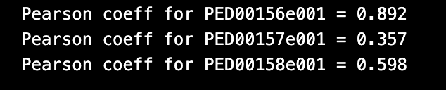
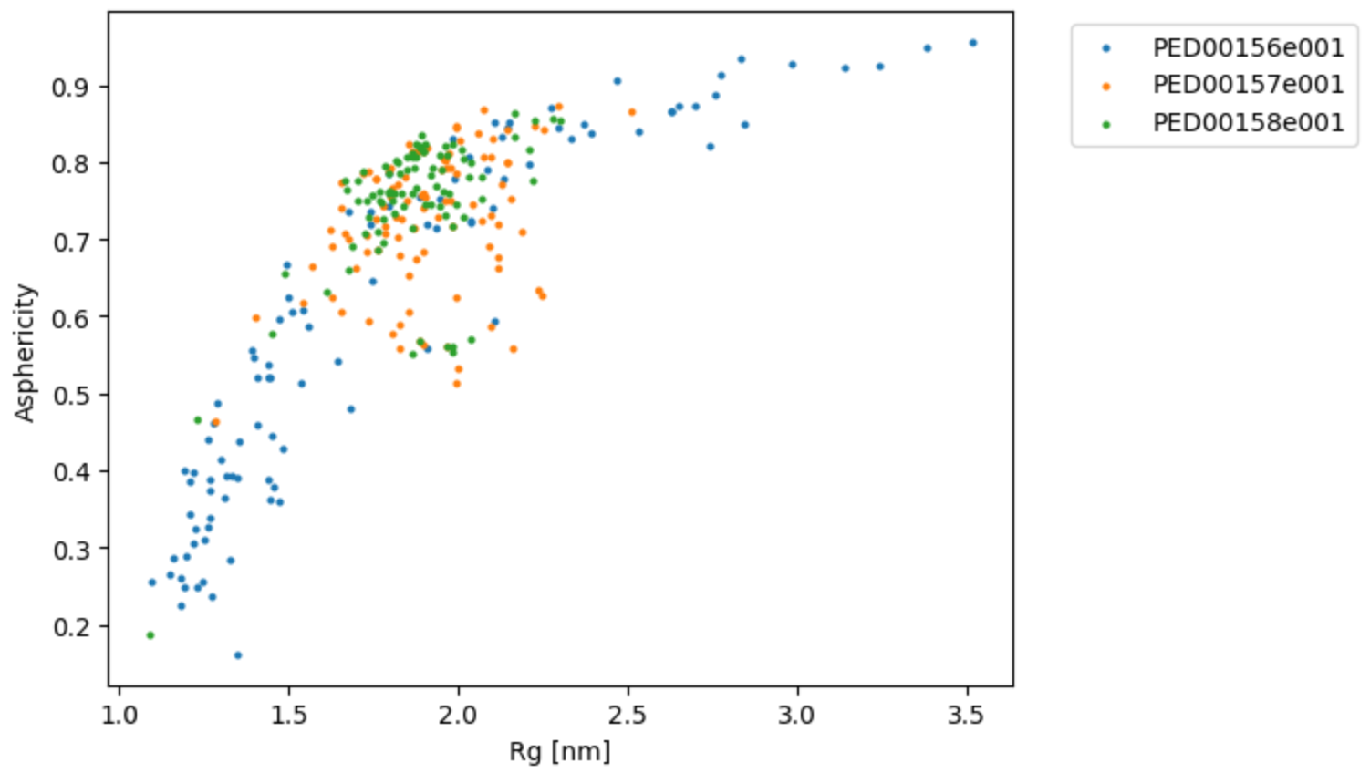
The function rg_vs_asphericity also prints the Pearson correlation coefficients, which measure the strength and direction of the linear relationship between the radius of gyration (Rg) and asphericity. A Pearson coefficient value close to 1 or -1 indicates a strong positive or negative correlation, respectively, while a value close to 0 indicates a weak or no correlation.
“save”: If True, saves the plot as an image file; default is False.
“ax”: The matplotlib Axes object on which to plot; if None, creates a new figure and axes.
vis.rg_vs_asphericity()
Radius of gyration vs Prolatness
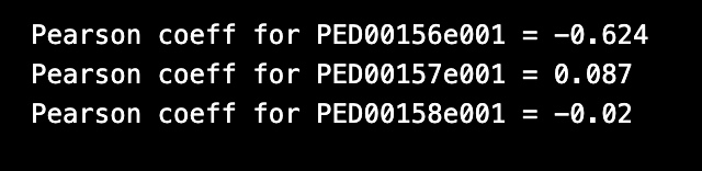
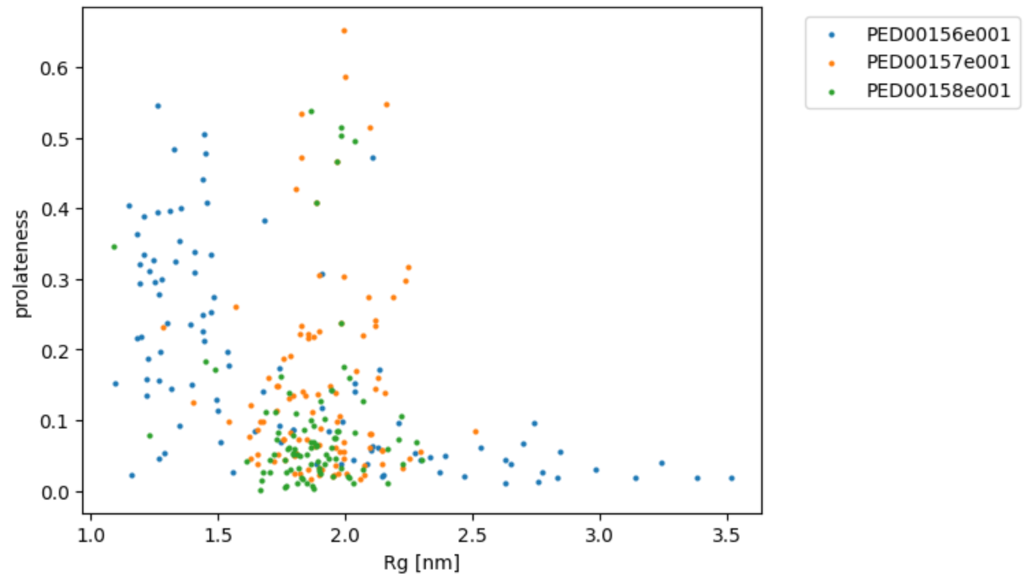
The function rg_vs_prolateness also prints the Pearson correlation coefficients, which measure the strength and direction of the linear relationship between the radius of gyration (Rg) and prolateness. A Pearson coefficient value close to 1 or -1 indicates a strong positive or negative correlation, respectively, while a value close to 0 indicates a weak or no correlation.
vis.rg_vs_prolatness()
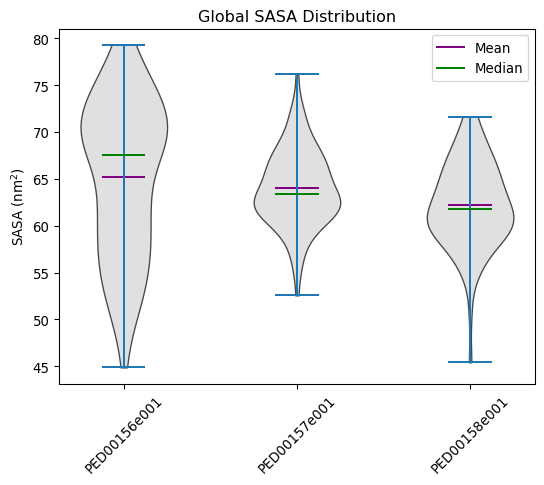
Global sasa distribution
The acronym ‘SASA’ stands for ‘Solvent Accessible Surface Area,’ which denotes the surface area of a molecule that is accessible to the solvent. The Shrake-Rupley algorithm implemented in MDTraj calculates SASA based on the positions of atoms and the specified probe radius. This algorithm partitions the molecular surface into a grid and computes areas accessible to solvent molecules. At the conformational level, ‘total SASA’ quantifies the overall surface area accessible to the solvent for each molecular conformation in the trajectory. At the residue level, SASA is computed by summing the solvent-accessible surface areas of all residues, offering insights into individual residue accessibility to the solvent.
“bins”: Number of bins for the histogram; default is 50.
“hist_range”: A tuple defining the min and max values for the histogram; if None, uses the data range.
“violin_plot”: If True, displays a violin plot; default is True.
“location”: It allows you to specify whether to calculate and use the mean (‘mean’) or the median (‘median’) as the reference value.
“save”: If True, saves the plot in the data directory; default is False.
“multiple_hist_ax”: If True, plots each histogram on a separate axis.
“ax”: The matplotlib Axes object on which to plot; if None, creates a new Axes object.
vis.ensemble_sasa(violin_plot=True, location='both', color='lightgrey')
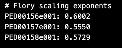
Flory scaling exponents
The Flory exponent is related to both the radius of gyration (Rg) and the end-to-end distance (Ree) of the polymer chain. For an ideal polymer chain at equilibrium—where residue-residue, residue-solvent, and solvent-solvent interactions are balanced—ν = 0.5, signifying a Gaussian chain structure. Deviations from this value indicate different conformational states:
ν < 0.5: A more compact structure. ν > 0.5: A more extended structure. As detailed in the paper [https://doi.org/10.1038/s41586-023-07004-5], Flory scaling exponents (ν) were determined by fitting the mean-squared residue-residue distances (⟨R²⟩) for sequential separations greater than five residues along the linear sequence. This approach is key to capturing the polymer-like behavior of proteins.
The analysis highlights the importance of ν in understanding the compaction of IDRs and its biological relevance. For example, proteins with compact IDRs (lower ν values) are often involved in crucial functions such as binding to chromatin and DNA cis-regulatory sequences. This suggests that IDR compaction plays a pivotal role in protein functionality and phase behavior.
v_values = analysis.get_features("flory_exponent")
for code in v_values:
print(f"{code}: {v_values[code]:.4f}")
Summary
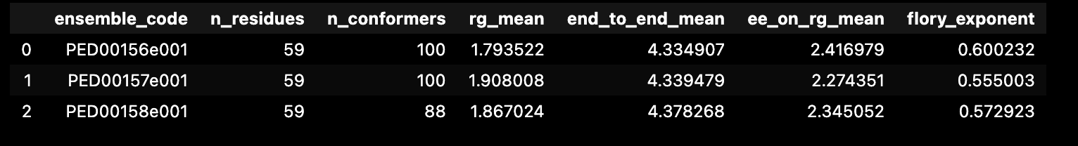
This code snippet calculates and displays a summary of features for each analyzed dataset. The function get_features_summary_dataframe is used to create a summary DataFrame that includes information about the selected key parameters.
In the provided example, the following parameters are selected: radius of gyration (rg), end-to-end distance (end_to_end), end-to-end distance to radius of gyration ratio (ee_on_rg), and Flory exponent (flory_exponent). This DataFrame is then displayed using the display(summary) statement.
selected_features : List of feature extraction methods to be used for summarizing the ensembles. Default is [“rg”, “asphericity”, “prolateness”, “sasa”, “end_to_end”, “flory_exponent”].
show_variability : If True, include a column a measurment of variability for each feature (e.g.: standard deviation or error).
analysis.get_features_summary_dataframe(selected_features=["rg", "end_to_end", "ee_on_rg", "flory_exponent"],show_variability=False)